Borrowing some ideas from document search techniques, data from the Shodan database can be used to characterize networks at a glance. In the last post, I used Shodan data for public IP spaces associated with different organizations and Wordle to create a quick and dirty word cloud visualization of exposure by port/service for that organization.
The word cloud idea works pretty well in communicating at a glance the top two or three ports/services most frequently seen for a given area of study (IP space). I wanted to extend this a bit and compare organizations by a linear rank of the most frequently occurring services seen on that organization’s network. So I wanted to capture both the most frequently occurring ports/services as well as the rank amongst those and then use those criteria to potentially compare different organizations (IP spaces).
Vector space model
I also wanted to experiment with visualizing this in a way that would give at a glance something of a ‘signature’. Sooooo, here’s the idea: document search often uses this idea of a vector space model where documents are broken down into vectors. The vector is a list of words representing all of the words that occur in that document. The weight given to each word (or term or element) in the vector can be computed in a number of different ways, but one of the most popular is frequency with which that word occurs in that document (and sometimes with which it occurs in all of the documents combined).
A similar idea was used here, except that I used frequency with which ports/services appeared in an organization instead of words in a document. I looked at the top 5 ports/services that appeared. I also experimented with the top 10 ports/services, but that got a little busy on the graphic and it also seemed that as I moved further down the ordered port list — 8th most frequent, 9th most frequent, etc — that these additional ports were adding less and less to the characterization of the network. Could be wrong, but it just seemed that way at the time.
I went through 12 organizations and collected the top 5 ports/services in each. Organizations varied between approximately 10,000 and 50,000 IP addresses. To have a basis for comparison of each organization, I used a list created by the ports returned from all of the organizations’ Top 5 ports.
Visualizing port rank ‘signatures’
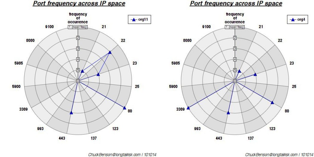
A polar plot was created where each radial represents each port/service. The rings of the plot represent the rank of that port — most frequently occurring, 2nd most frequently occurring, …, 5th most frequently occurring. I used a polar plot because I wanted something that might generate easily recognizable shapes or patterns. Another plot could have been used, but this one grabbed my eye the most.
Finally, to really get geeky, to measure similarity in some form, I computed the Euclidean distance between each possible vector pair. Two of the closest organizations of the 12 analyzed are (that is most similar port vectors):

2 of the most similar organizations by Euclidean distance — ports 21, 23, & 443 show up with the same rank & port 80 shows up with a rank difference of only 1. This makes them close. (Euclidean distance of ~2.5)
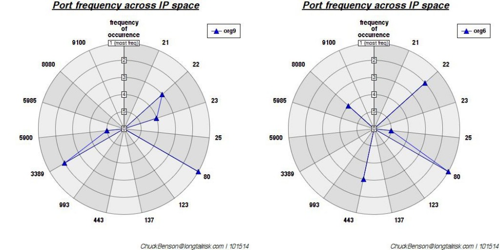
Two of the furthest way of the 12 studied are these (least similar port vectors):

While port 80 aligns between the two (has the same rank) and port 22 is close in rank between the two, there is no alignment between ports 23, 3389, or 5900. This non-alignment, non-similar port rank, creates more distance between the two. (Euclidean distance of ~9.8)
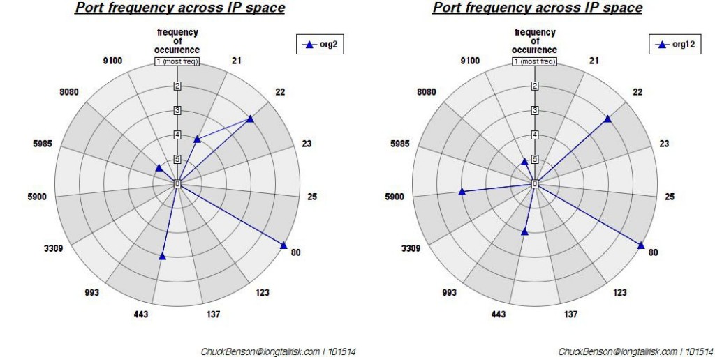
Finally, this last one is some where in the middle (mean) of the pack:

A distance chosen from the middle of the sorted distance (mean). Euclidean distance is ~8.7. Because this median value is much closer to the most dissimilar, it seems to indicate a high degree of dissimilarity across the set studied (I think).
Overall, I liked the plots. I also liked the polar approach. I was hoping that I would see a little more of a ‘shape feel’, but I only studied 12 organizations. I’d like to add more organizations to the study and see if additional patterns emerge. I also tried other distance measuring methods (Hamming, cosine, jaccard, Chebyshev, cityblock, etc) because they were readily available and easy to use with the scipy library that I was using, but none offered a noticeable uptick in utility over the plain Euclidean measure.
Cool questions from this to pursue might be:
1. For similar patterns between 2 or more organizations, can history of network development be inferred? Was a key person at both organizations at some point? Did one org copy another org?
2. Could the ranked port exposure lend itself to approximating risk for combined/multiprong cyber attack?
Again, if you’re doing similar work on network/IP space characterization and want to share, please contact me at ChuckBenson at this website’s domain for email.

